統計検定2級の勉強をする話⑧

前回↓
今回は2変数の確率分布、標本分布、中心極限定理について
2変数の確率分布
同時確率分布
2つの確率変数X、Yの取りうる値と確率の対応関係を同時確率分布といい、定義される関数を同時確率関数という。
\[ P(X = x_i, Y = y_j) = p(x_i, y_j) \]
その中で片方の確率分布を示したものを周辺分布といい、その関数を周辺確率関数という。
\[ P(X = x_i) = \sum_j p(x_i, y_j) \]
2つの確率変数の共分散、相関係数
同時確率分布の期待値はそれぞれの確率変数の期待値の和に等しい。
\[ E[X + Y] = E[X] + E[Y] \]
なので分散は
\[ \text{Var}(X + Y) = \text{Var}(X) + \text{Var}(Y) + 2(E[XY] - E[X]E[Y]) \]
となる。ここで第3項が共分散
\[ \text{Covariance} =2(E[XY] - E[X]E[Y]) \]
であり、共分散とそれぞれの分散から相関係数が導ける。
\[ \rho(X, Y) = \frac{\text{Covariance}(X, Y)}{\sqrt{\text{Var}(X) \cdot \text{Var}(Y)}} \]
2変量正規分布
2つの連続型確率関数が正規分布に従うとき、その同時確率密度関数は
\[ f(x, y) = \frac{1}{2\piσ_Xσ_Y\sqrt{1-\rho^2}} \exp\left(-\frac{1}{2(1-\rho^2)}\left[\frac{(x-\mu_X)^2}{σ_X^2} + \frac{(y-\mu_Y)^2}{σ+_Y^2} - \frac{2\rho(x-\mu_X)(y-\mu_Y)}{σ_Xσ_Y}\right]\right) \]
で表される
これを3次元上で示すと、あらゆるx、yの条件付き分布が正規分布に従うことがわかる。
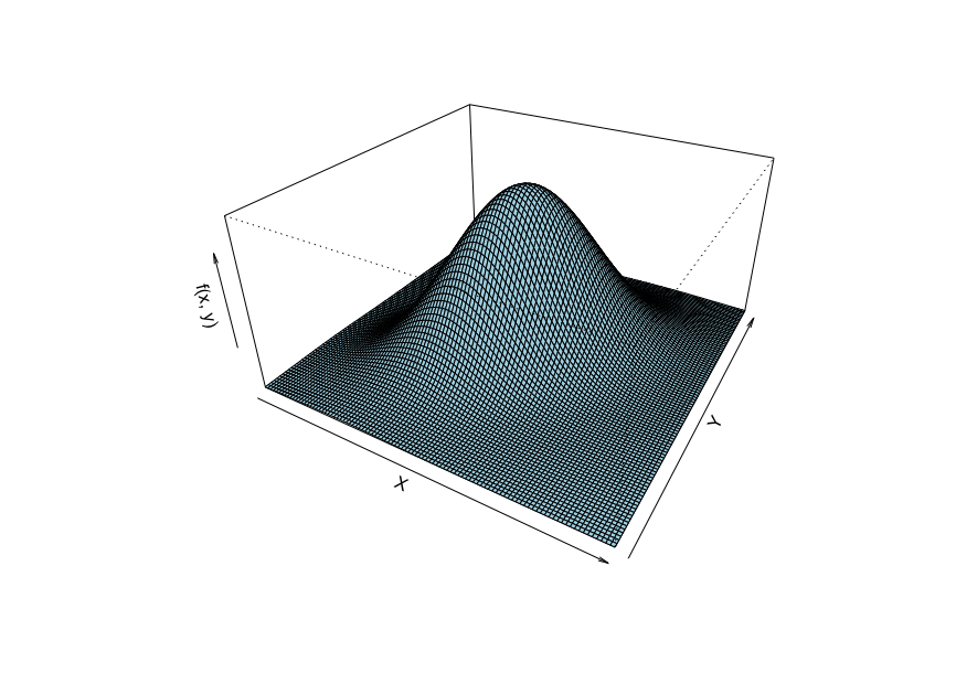
その正規分布の期待値と分散は
\[ E[Y | X = x] = \mu_Y + \rho \frac{σ_Y}{σ_X} (x - \mu_X) \]
\[ \text{Var}(Y | X = x) = σ_Y^2 (1 - \rho^2) \]
標本分布
母集団から無作為標本を抽出したときの統計量の確率分布を標本分布という。
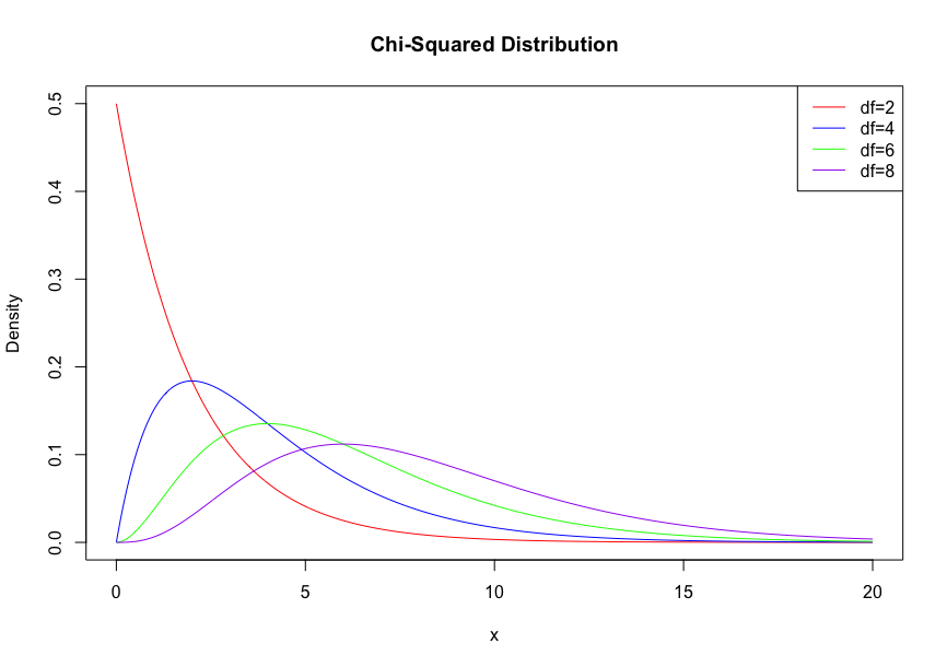
\( χ^2\)分布
複数の確率変数が互いに独立で、標準正規分布に従うときのそれぞれの確率変数の2乗の和の分布。
確率変数の数nを自由度という。
その期待値と分散は
\[ E[X] = n \]
\[ \text{Var}(X) = 2n \]
となる
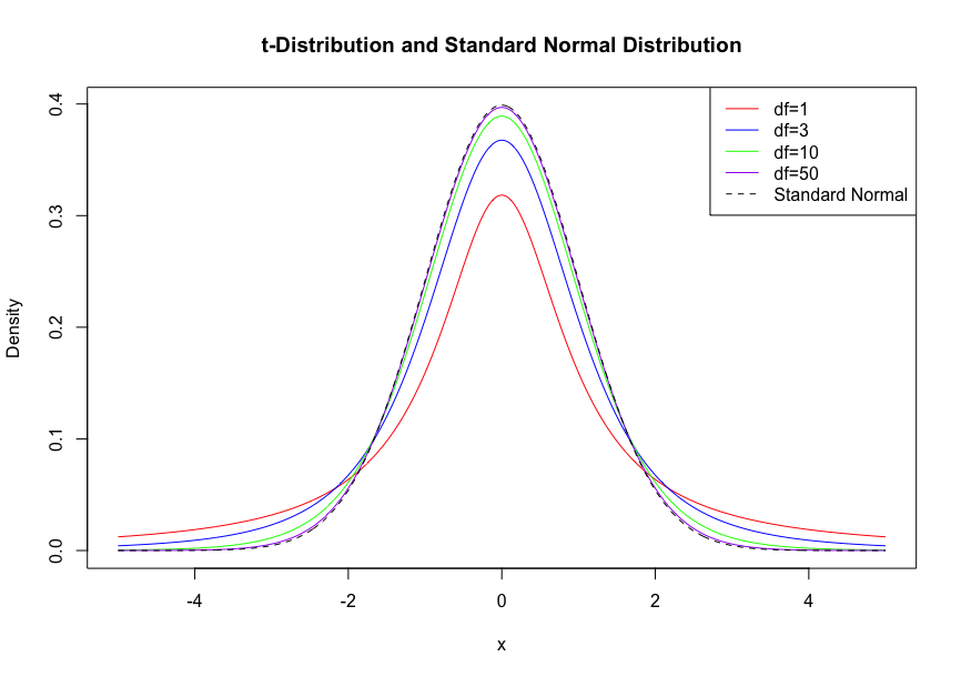
t分布
独立な2つの確率変数において、片方が標準正規分布、もう片方が自由度nの\( χ^2\)分布に従う時、
\[ t = \frac{Z}{\sqrt{W/n}} \]
の分布をt分布という。
その期待値、分散は
\[ E[T] = \begin{cases} 0 & \text{if } n > 1 \\ \text{undefined} & \text{if } n \leq 1 \end{cases} \]
\[ \text{Var}(T) = \begin{cases} \frac{n}{n - 2} & \text{if } n > 2 \\ \infty & \text{if } 1 < n \leq 2 \\ \text{undefined} & \text{if } n \leq 1 \end{cases} \]
自由度を大きくすると標準正規分布に近づく
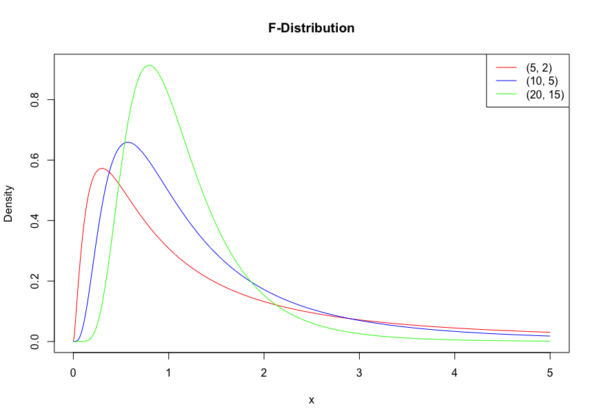
F分布
独立に自由度N1、N2の\( χ^2\)分布に従う確率変数W1、W2がある時、
\[ F = \frac{W_1/N_1}{{W_2/N_2}} \]
の従う分布をF分布という。
大数の法則と中心極限定理
なんか結構前に一回勉強した気がするからざっくり。
大数の法則(弱法則)
以下に示すチェビシェフの不等式は任意の確率変数に対して、上限と下限を設けることができる。
\[ P(|X - \mu| \geq kσ) \leq \frac{1}{k^2} \]
これを標本平均に対して考え、nを無限に大きくすると、
\[ \forall \epsilon > 0, \lim_{{n \to \infty}} P\left(|\bar{X}_n - \mu| \geq \epsilon\right) = 0 \]
となり、標本平均は母平均に収束する。
中心極限定理
nが大きい場合、元の分布が正規分布に従わない場合でもその平均は正規分布に近づく。
そして母集団の平均がμ、標準偏差がσ、標本サイズがnの時標本集団の平均はμ、標準偏差σ/√nに従う。
今日はここまで。
標本分布に関してはイマイチどう実用できるのかわからん。
Study for Statistics Test Level 2 (7)
previous page↓
Today's study is about specific distributions.
Discrete probability distributions
Bernoulli distribution
A trial is termed a "Bernoulli trial" when the outcomes are independent of each other and have the same probability.
When only one Bernoulli trial is conducted, and there are two possible outcomes, the resulting distribution is called a "Bernoulli distribution." Its probability function is defined as:
\[ P(X = k) = p^k (1 - p)^{1 - k} \]
Binomial distribution
A "Binomial distribution" arises when one outcome occurs times and the other outcome occurs times in Bernoulli trials.
The probability function for a binomial distribution is defined as:
\[ P(X = k) = \frac{n!}{k! (n - k)!}p^k (1 - p)^{n - k} \]
expectation:\[ \mu = np \]
variation:\[ σ^2 = np(1 - p) \]
standard deviation:\[ σ = \sqrt{np(1 - p)} \]
Poisson distribution
In a binomial distribution, when the expectation is defined as a specific value, and approaches infinity while approaches zero, the resulting distribution is termed a "Poisson distribution."
The Poisson distribution serves as a useful probability model for events that occur rarely.
probability function:\[ P(X = k) = \frac{\lambda^k e^{-\lambda}}{k!} \]
expectation:\[ \mu = \lambda \]
variation:\[ σ^2 = \lambda \]
Geometric distribution
A geometric distribution describes the number of Bernoulli trials needed for the first success.
probability function:\[ P(X = k) = (1 - p)^{k - 1} p \]
expectation:\[ \mu = \frac{1}{p} \]
variation:\[ σ^2 = \frac{1 - p}{p^2} \]
Continuous probability distributions
Uniform distribution
A uniform distribution has equal probability across the range of to .
probability density function:\[ f(x) = \begin{cases} \frac{1}{b - a} & \text{for } a \leq x \leq b, \\ 0 & \text{otherwise.} \end{cases} \]
expectation:\[ \mu = \frac{a + b}{2} \]
variation:\[ σ^2 = \frac{(b - a)^2}{12} \]

Normal distribution(Gaussian distribution)
When the expectation and variance are defined, the probability function of a normal distribution is given as:
probability density function:\[ f(x) = \frac{1}{σ\sqrt{2\pi}} e^{-\frac{1}{2} \left(\frac{x - \mu}{σ}\right)^2} \]
standardization:\[ z = \frac{x - \mu}{σ} \]

If random variables follow a normal distribution, their sum also follows a normal distribution.
Exponential distribution
The exponential distribution represents the time until the first event occurs in a Bernoulli trial.
probability density function:\[ f(x) = \lambda e^{-\lambda x} \text{ for } x \geq 0, \text{ and } 0 \text{ otherwise.} \]
expectation:\[ \mu = \frac{1}{\lambda} \]
variation:\[ σ^2 = \frac{1}{\lambda^2} \]

Today's study has concluded.
統計検定2級の勉強をする話⑥
前回
統計を勉強し始めてから基本的な数学知識を忘れている(そもそも身につけていない)ことに気づいて、高校の教科書を眺めている。何も思い出せん。
本日は「確率変数と確率分布」
確率変数(random variable)
変数Xの値はわからないが、その値になる確率が与えられているとき、Xを確率変数という。また、取りうる値と確率の対応を確率分布という。
離散型確率変数
サイコロの目のようにXの値が離散的値を取る時、離散型確率変数と言う。
サイコロの目のようにどの値に対しても確率が同一である時、離散一様分布という。
連続型確率分布
連続値を取る時の確率変数は上記の方法だと無限に発散してしまう。
ので、任意のΔxに対して積分して、
Xが区間[a,b]を取る確率を
\[ P(a \leq X \leq b) = \int_{a}^{b} f(x) \, dx \]
を表す。
確率関数(probability function)
確率変数 \( X \) が値 \( x \) を取る確率を示すと
\( p(x) = P(X = x) \)
となり、これを確率関数という。
ここで、
\[ 0 \leq p(x) \leq 1 \]
\[ \sum_{x} p(x) = 1 \]
となる。
累積分布関数
離散型、連続型どちらの確率変数に対しても累積分布関数が\[ P(X \leq x) \]で定義される。
連続型の場合は、
\[ F(x) = P(X \leq x) = \int_{-\infty}^{x} f(t) \, dt \]
で定義できる。
期待値
確率変数がどのような値を取ることが期待されるか(日本語合ってる?)を示す値
離散型の場合
\( E(X) = \sum_{i} x_i P(X = x_i) \)
連続型の場合
\( E(X) = \int_{-\infty}^{\infty} x f(x) \, dx \)
分散
期待値は母集団分布の平均と考えることができるので、その偏差をとって分散を定義できる。
離散型の場合
\( \text{Var}(X) = \sum_{i} (x_i - E(X))^2 P(X = x_i) \)
連続型の場合
\( \text{Var}(X) = \int_{-\infty}^{\infty} (x - E(X))^2 f(x) \, dx \)
また式変形すると以下のようにも表せる。
\[ \text{Var}(X) = E[X^2] - (E[X])^2 \]
モーメント
確率変数\( X^k \)の期待値をk次のモーメントという。
\( (X-μ)^k \)の期待とをk次の中心モーメントという。
k=1,2のモーメントは分布の中心の位置と散らばりの大きさを示す。
k=3の中心モーメントを標準偏差の3乗で割った値\[ \text{Skewness}(X) = \frac{E[(X - \mu)^3]}{σ^3} \]を歪度と言う。
歪度は分布の非対称さを表していて、対称なら0、右に長い裾を持つと正、左に長い裾を持つと負の値をもつ。
k=4の中心モーメントは分布の尖り具合を示し、尖度という。正規分布の値である3を引いて
\[ \text{Kurtosis}(X) = \frac{E[(X - \mu)^4]}{σ^4} - 3 \]
と定義する。
正規分布より裾が長い場合は正、短い場合は負の値を取る。
本日はここまで〜
次回からは具体的な確率分布が出てくるようだが、数式がたくさん並んでいて辛い。
Study for Statistics Test Level 2 (5)
previous page↓
Today's Study: Probability
Terms:
- Trial: An experiment or observation that results randomly.
- Elementary Event: Each result of a trial.
- Event: A set of elementary events.
- Whole Event: The set of all elementary events.
- Union: When at least one result occurs in several events. Denoted as: \[ A \cup B \]
- Intersection: When each event occurs at the same time. Denoted as: \[ A \cap B \]
- Empty Set or Null Set: The event where nothing occurs. Denoted as: \[ \emptyset \]
- Complement: The event excluded from a particular event in the whole event. Denoted as: \[ A^c \]
- Mutually Exclusive: When the intersection between two events is an empty set.
Definition of Probability:
Probability is a function defined with the following features:
Kolmogorov's Axioms:
- For any event \( A \), the probability is non-negative and does not exceed 1: \[ 0 \leq P(A) \leq 1 \]
- The probability of the sample space \( S \) is 1: \[ P(S) = 1 \]
- For any sequence of mutually exclusive events \( A_1, A_2, \dots \): \[ P\left( \bigcup_{i=1}^{\infty} A_i \right) = \sum_{i=1}^{\infty} P(A_i) \]
Specific Definitions:
Laplace's Definition of Probability:
The probability \( P(A) \) of an event \( A \) is given by: \[ P(A) = \frac{n(A)}{n(S)} \] where \( n(A) \) is the number of favorable outcomes for event \( A \) and \( n(S) \) is the total number of possible outcomes.
Frequency-based Definition of Probability:
The probability \( P(A) \) of an event \( A \) is given by: \[ P(A) = \lim_{{n \to \infty}} \frac{m}{n} \] where \( m \) is the number of times event \( A \) occurs in \( n \) trials.
Theorems of Probability:
Addition Theorem of Probability:
The probability \( P(A \cup B) \) of the union of events \( A \) and \( B \) is given by: \[ P(A \cup B) = P(A) + P(B) - P(A \cap B) \] where \( P(A \cap B) \) is the probability that both events \( A \) and \( B \) occur.
Conditional Probability:
Given an event \( B \), the conditional probability of event \( A \) is: \[ P(A|B) = \frac{P(A \cap B)}{P(B)} \] where \( P(B) > 0 \).
Multiplication Theorem:
The probability of the intersection of events \( A \) and \( B \) is: \[ P(A \cap B) = P(A|B) \times P(B) \] or \[ P(A \cap B) = P(B|A) \times P(A) \]
Bayes' Theorem :
The probability of event \( A_i \) given event \( B \) is: \[ P(A_i|B) = \frac{P(B|A_i) \times P(A_i)}{\sum_{j} P(B|A_j) \times P(A_j)} \] where:
- \( A_i \) is a specific event from the set of possible events \( \{A_1, A_2, \dots\} \).
- The summation over \( j \) represents the sum over all possible events \( A_j \).
統計検定2級の勉強をする話④

前回↓
今回は日本語で。
「時系列データ」の話。
時系列データの扱い
ある時刻 t → t+1 におけるyの変化を見る方法は
- 差を見る(yt+1 - yt )
- 変化率を見る((yt+1 - yt )/yt)
の二種類が基本的である。
指数化
ある時点sを基準点とし、
qt = yt/ys
という指数の推移を見る方法。
西暦末尾0 or 5年の値の平均値を基準とすることが多い。
比で変化を見る方法
前期比は
rt=yt/yt-1
とすることができる。
平均の伸び率を計算する場合は算術平均ではなく幾何平均
\( \sqrt[n]{x_1 \times x_2 \times \ldots \times x_n} \)
を用いる。
変動分解
時系列データの時間的変動は以下の2種類に分けることができる。
- 傾向変動(TC):長期に渡る動きを表す変動
- 季節変動(S):1年を周期として循環を繰り返す変動
- 不規則変動( I ):上記以外の変動
つまりある時点tの時系列データに関して、
yt=TCt+St+It
と分解できる.
TCtの抽出
移動平均法(moving average method)
ある時点tとその前後±kの間の2k+1個の値に対して移動平均は
\[ \hat{TC}_t = \frac{1}{2k+1} \sum_{i=t-k}^{t+k} Y_i \]
で求められ、周期2k+1で循環する成分を除去できる。
*周期が偶数の場合はk+1とk-1時点の値を1/2にして無理やり奇数にして計算する。
Stの計算
傾向変動成分を引いた時系列データWは
Wt = yt - TCt = St+It
で、季節変動と不規則変動を含んでいる。
月毎のWの平均を取り、月別の平均からW全体の平均を引く
自己相関
時刻tの時系列とtからhずらしたt+hの時系列の相関関係を考える。
この時相関係数rhは自己共分散関数(autocovariance function)を用いて計算する。
自己共分散関数 (Autocovariance Function):
\[ \gamma(h) = \frac{1}{n} \sum_{t=1}^{n-h} (X_t - \bar{X})(X_{t+h} - \bar{X}) \]
自己相関係数 (Autocorrelation Function):
\[ \rho(h) = \frac{\gamma(h)}{\gamma(0)} \]
横軸にラグh、rhを縦軸にしたグラフをコレログラムと言い、相関の強い周期を可視化できる。
本日はここまで。
数学の知識が足りなくて辛い。勉強しとけばよかった。
Study for Statistics Test Level 2 (3)
previous page
Today's study is about 'dealing with qualitative data' and 'statistics and summary of double variable data'.
Dealing with qualitative data
The method of visualizing qualitative data is either a bar graph or a pie chart. If you use an ordinal scale, you should arrange data from smallest to largest.

There's a bar graph using the Titanic ML from the disaster and a pie chart using the same dataset.
Statistics and summary of double variable data
Scatter diagram
Scatter plots are helpful to confirm correlation. The more one variable increases, the more the other increases in a positive correlation. Conversely, the more one variable increases, the more the other decreases in a negative correlation. With neither of these correlations, it is termed as no correlation. Correlation has strength.
Cross table
If you have a lot of data, you can separate the quantity variable into several classes. Cross tables display the frequency in these classes. Marginal frequencies are counted in every class for each variable.
Correlation coefficient
Covariance
$$ \text{Covariance} = \frac{\sum{(X_i - \bar{X})(Y_i - \bar{Y})}}{n} $$
The formula for the Pearson correlation coefficient divides covariance by SD:
\( r = \frac{n(\sum xy) - (\sum x)(\sum y)}{\sqrt{[n\sum x^2 - (\sum x)^2][n\sum y^2 - (\sum y)^2]}} \)
If these values are positive, there's a positive correlation. If negative, there's a negative correlation. The correlation coefficient ranges between -1 and 1. It also represents the covariance of the z-score.
*Attention
Correlation does not imply causation. When there's correlation but not causation, the correlation is termed 'spurious correlation'. For instance, a third value can affect the correlation coefficient. The correlation coefficient indicates only a linear relation, not a non-linear relation.
Partial correlation
When a third value affects the correlation coefficient, it's necessary to remove the effect of the third value for precise correlation, termed 'partial correlation'. The formula for the partial correlation coefficient between variables X and Y, controlling for variable Z, is:
\( r_{XY.Z} = \frac{r_{XY} - r_{XZ} r_{YZ}}{\sqrt{(1 - r_{XZ}^2)(1 - r_{YZ}^2)}} \)
Where:
- \( r_{XY} \) is the correlation coefficient between \(X\) and \(Y\).
- \( r_{XZ} \) is the correlation coefficient between \(X\) and \(Z\).
- \( r_{YZ} \) is the correlation coefficient between \(Y\) and \(Z\).
Regression line
The regression line is used to predict Y from X. X is defined as the explanatory variable, and Y is defined as the response variable. Consider the relationship as "Y = α+βx". This line is termed the "Regression line", and α and β are known as "regression coefficients".
The formula for the Error Sum of Squares (ESS) is:
\( \sum_{i=1}^{n} (y_i - \hat{y}_i)^2 \)
Where:
- \( y_i \) is the actual observed value.
- \( \hat{y}_i \) is the predicted value from the model.
- \( n \) is the number of data points.
\( y_i - \hat{y}_i \) is termed "residual".
The Least Squares Method seeks the regression coefficient when ESS is at its minimum.
On the regression line, there are several key features:
- The mean of the predicted value equals the mean of the response variable.
- The mean of the residual is zero.
- The regression line passes through (\( \bar{x}, \bar{y} \)).
- The correlation coefficient between prediction and residual is zero.
- The Total Sum of Squares breaks down into Regression Sum of Squares and Residual Sum of Squares.
- Dividing the Regression Sum of Squares by the Residual Sum of Squares is termed the "coefficient of determination (\( R^2 \))". \( R^2 \) ranges from zero to one. When \( R^2 \) is one, the regression line fully explains the actual observed value.
Today's study has finished.
…英語難しい。。。
Rを触ってみる話②
前回↓
今回はパッケージについて。
なんか意外とRがPythonの知識で動かせて嬉しい。
パッケージのダウンロード、インストール
今回は'ggplot2'をインストールする。matplotlib的なやつか?
install.packages("ggplot2")でインストール
library("ggplot2")でロード
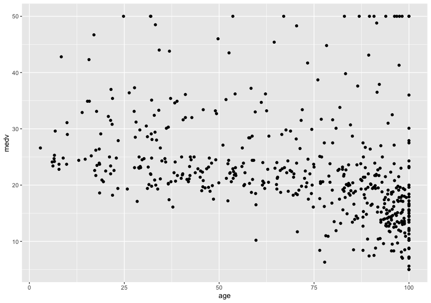
散布図
gplot内のqplotを使ってみる。(quick plotの略らしい)
qplot(Boston'age', Boston'medv')
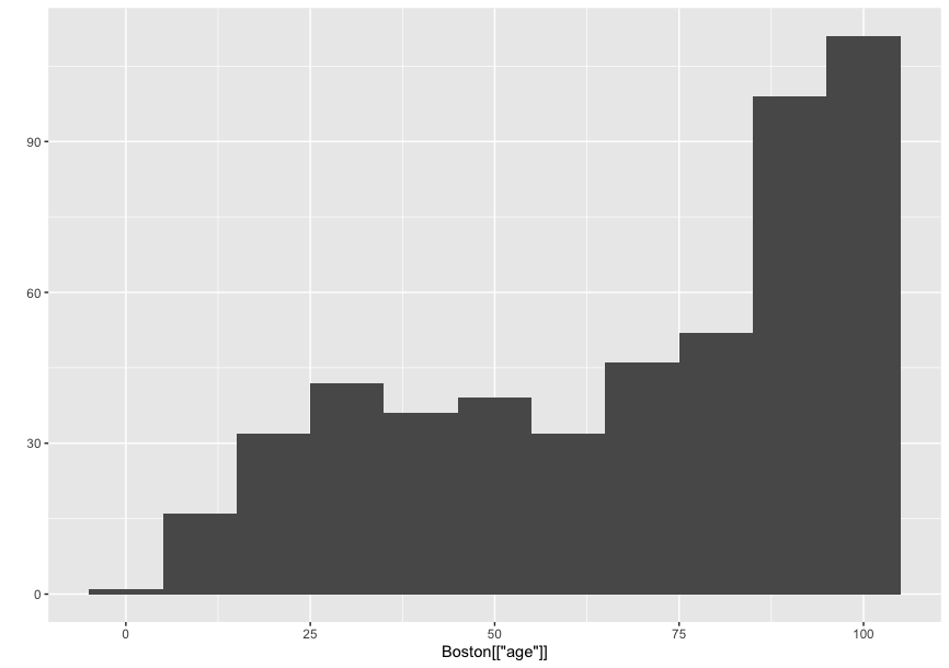
ヒストグラム
引数一つにしたらいいだけ
qplot(Boston'age')
ここで、データフレームの特定の列を取り出すのに[]を使っていたのだが、$で表せることを知る。RStudioで予測変換的なの出るし。
python的には使いたい感あるが$が便利すぎるのでそっちを使う。
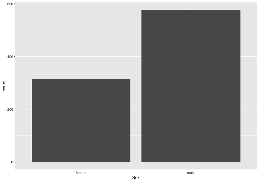
棒グラフ
なんかこの関数を+で足してく感じがいまいち慣れない。
frequency <- as.data.frame(table(train$Sex))
ggplot(frequency, aes(x=Var1, y=Freq)) +
geom_bar(stat="identity")

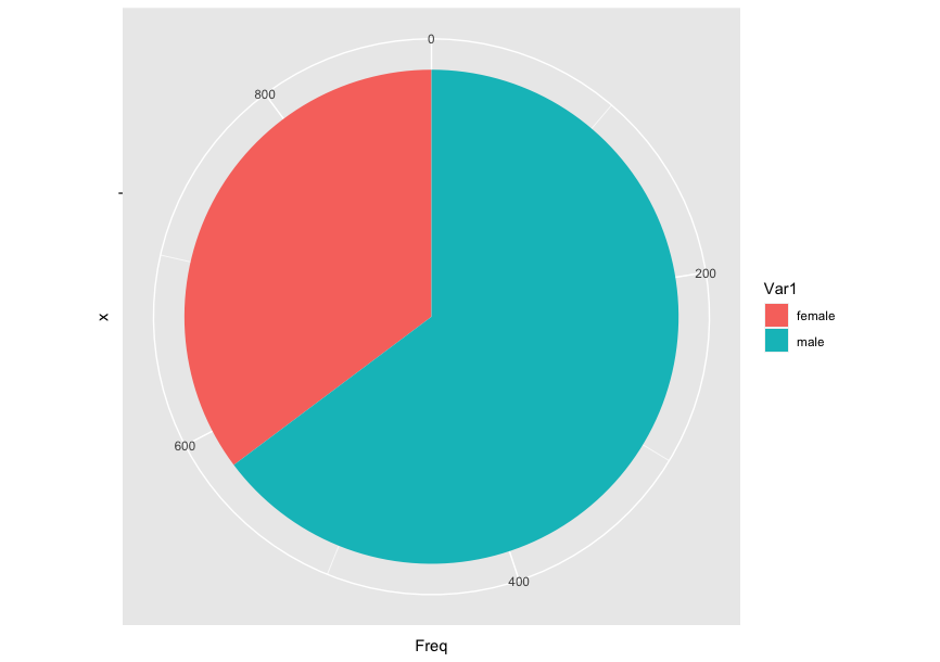
円グラフ
frequency <- as.data.frame(table(train$Sex))
ggplot(data, aes(x="", y=Freq, fill=Var1)) +
geom_bar(width = 1, stat = "identity") +
coord_polar("y", start=0)
クロス集計表
breaksにリストを入れればその範囲ごとに区切るし、整数を渡せば均等に切ってくれる。
ageGroup <- cut(Boston$age, breaks = 10)
medvGroup <- cut(Boston$medv, breaks = 10)
> table(ageGroup, medGroup)
medGroup
ageGroup (4.96,9.5] (9.5,14] (14,18.5] (18.5,23] (23,27.5] (27.5,32] (32,36.5] (36.5,41] (41,45.5] (45.5,50]
(2.8,12.6] 0 0 0 1 9 3 0 0 1 0
(12.6,22.3] 0 0 1 8 10 3 6 1 1 1
(22.3,32] 0 0 1 7 9 6 2 1 0 3
(32,41.7] 0 0 2 15 7 8 7 0 2 1
(41.7,51.4] 0 0 1 17 9 1 3 0 0 1
(51.4,61.2] 0 1 3 16 8 3 4 1 1 1
(61.2,70.9] 0 1 3 20 5 5 2 0 1 2
(70.9,80.6] 2 3 6 14 9 4 1 1 2 0
(80.6,90.3] 3 6 16 27 9 3 1 2 1 3
(90.3,100] 17 44 52 29 9 3 3 1 1 9
なんかズレた。
まだ慣れない。というか慣れてるpythonでやった方が早い。
続く。