機械学習の評価指標を学ぶ

統計検定も落ち着いたので、ぼちぼち機械学習の勉強も再開したい。
こちら過去五年のKaggleコンペの主要指標
- LogLoss
- AUC
- WeightedMeanColumnwiseLogLoss
- QuadraticWeightedKappa
- OpenImagesObjectDetectionAP
- MWCRMSE
- MCAUC
- MAP@K
- Jaccard
回帰問題の評価指標
RMSE:Root Mean Squared Error
$$ \text{RMSE} = \sqrt{\frac{1}{n} \sum_{i=1}^{n} (y_i - \hat{y}_i)^2} $$
平均二乗誤差の平方根。
def rmse_sklearn(predictions, targets):
    mse = mean_squared_error(targets, predictions)
    return np.sqrt(mse)
*外れ値の影響を受けやすい
*目的変数の平方根をとってMSEを目的関数として学習して適合できる
RMSLE:Root Mean Squared Logarithmic Error
$$ \text{RMSLE} = \sqrt{\frac{1}{n} \sum_{i=1}^{n} (\log(1 + y_i) - \log(1 + \hat{y}_i))^2} $$
予測値と実測値の対数の差の二乗の平均の平方値
def rmsle(y_true, y_pred):
    return np.sqrt(mean_squared_log_error(y_true, y_pred))
*目的変数の対数を新たな目的変数としてRMSEを実施しているのと同じ。
*目的変数が裾の重い分布を撮る時に有用
*予測値の差は重要ではなく、尺度が実測値と同じかどうかが重要
MAE:Mean Absolute Error
$$ \text{MAE} = \frac{1}{n} \sum_{i=1}^{n} |y_i - \hat{y}_i| $$
実測値と予測値の差の絶対値の平均
def mae(actual, predicted):
    return np.mean(np.abs(actual - predicted))
*外れ値 の影響を受けにくい
*計算時間長くなりがち
*予測値=実測値で微分不可能なので勾配ブースティングなどが使用できない。
そのため損失関数には近似関数としてfair関数やPseudo-Huber関数を用いる必要がある。
<fair関数>
def fair_function(x, c=1.0):
    return c**2 * (np.abs(x)/c - np.log(1 + np.abs(x)/c))
<Pseudo-Huber関数>
def pseudo_huber_function(x, delta=1.0):
    return delta**2 * (np.sqrt(1 + (x/delta)**2) - 1)
二値分類の評価指標(正例である確率が予測値の場合)
logloss(cross entropy)
\[logloss = -\frac{1}{N} \sum_{i=1}^{N} [y_i \log(p_i) + (1 - y_i) \log(1 - p_i)]\]
正負の予測の確率をより大きく外すと損失が大きくなるようになっている
from sklearn.metrics import log_loss
loss = log_loss(y_true, y_pred)
AUC(Area Under the ROC curve)
ROC曲線の面積
予測値を正例とする閾値を1から0にしたときの偽陽性率と真陽性率をプロットしたグラフ
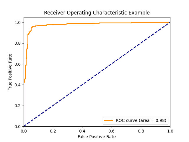
from sklearn.metrics import roc_auc_score
auc = roc_auc_score(y_true, y_pred)
*青点線は完全ランダムの場合で、AUCは0.5になる
*予測値の大小関係のみが影響するため、必ずしも確率である必要はなく、別の指標を用いても良い。
*負例の予測より正例の予測の誤差の方が影響を受けやすい。
*Gini係数とは線形関係
マルチクラス分類の評価指標
quadratic weighted kappa
クラス間に順序関係がある場合に用いる
$$ \kappa = 1 - \frac{\sum_{i,j}w_{ij}o_{ij}}{\sum_{i,j}w_{ij}e_{ij}} $$
from sklearn.metrics import cohen_kappa_score
kappa = cohen_kappa_score(rater1, rater2, weights='quadratic')
完全に予測すると1、ランダムだと0、それ以下だと負の値を取る。
レコメンデーションの評価指標
MAP@K
$$ MAP@K = \frac{1}{Q} \sum_{q=1}^{Q} \left( \frac{1}{\min(m_q, K)} \sum_{k=1}^{K} \text{Precision}(k) \times \text{rel}_q(k) \right) $$
def average_precision_at_k(actual, predicted, k):
    if not actual:
        return 0.0

    score = 0.0
    num_hits = 0.0

    for i, p in enumerate(predicted[:k]):
        if p in actual and p not in predicted[:i]:
            num_hits += 1.0
            score += num_hits / (i + 1.0)

    return score / min(len(actual), k)

def map_at_k(actual, predicted, k):
    return sum(average_precision_at_k(a, p, k) for a, p in zip(actual, predicted)) / len(actual)
*正解数が同じでも正解の順位が低いとスコアが下がる。
*K個の予測値を提示できる時にK個未満の予測をすることもできるがスコアは下がるのであまり意味はない
2ヶ月勉強して統計検定2級にギリギリ合格した話
本日は統計検定2級に合格した話です。
なんかこういう話って盛って話すとPV数稼げそうなので頑張って書きます。
統計検定2級
難易度
結論から言うと理系か文系で大きく異なる気がする。
HPによると統計検定2級のレベルは大学基礎課程レベルの統計学が問われる検定とのこと。大学基礎課程というと1.2年で勉強する内容のようなので、大学で統計学とってた人からすると余裕なのだろう。
私は統計学の授業はなかったがなんかの授業でt検定とかχ2乗検定とかが出てきたような記憶がある。しかし当時は試験で出る問題がすでに教えられていて、その回答を丸暗記するという何のしょうもない勉強をしていた。
と言うわけで実質数学は高校以来だが、(一応)理系だったので数列とか積分に耐性ができていて、アレルギー症状は出なかった。文系の方は一度高校数学の教科書を開いてみてアレルギー症状が出ないか負荷試験をお勧めする。数学アレルギーの人は多分苦行。
勉強時間
私の場合は効率重視で勉強しつつ後述する全く非効率的な勉強も混ぜていたので、
トータル50時間くらい。全部で2ヶ月かかったが、真面目にやったのは最後の2週間くらいなので、理系の方は1ヶ月以内でもいけそう。というのは働きながらの話なので、時間が取れればもっと早く取れるかも。
結果
あっぶな。 pic.twitter.com/WkOEX6uC0G
— でふぺど (@DefPediatr) October 29, 2023
くっそギリギリである。時間もジャストぐらいで見直す時間はなかった。
実際にやった勉強方法と感想
①公式テキストを読む
とりあえず出題範囲の確認も踏まえて公式テキストを読んだ。
合格するだけだったらこれと問題集だけでいけると思われる。
わかりにくいとのレビューが散見されるが、個人的には別に可もなく不可もない印象。
②公式問題集を解く
試験前2週間切ったあたりから公式問題集というのがあったので、それをやった。
CBT方式で受けるからCBTのやつだけでいいかと思っていたが、何となく問題数が足りない印象だったのでHPで公開されている2021年度の過去問もやった。
1週といて、わからない問題だけ2週した。ほんとは全体を2週したかったけど時間がなく断念。
③統計学入門をチラ見する
ネットでの評判が良かったので購入。
まぁわかりやすくはあるのだが、試験範囲と絶妙に噛み合わない部分もあるので問題集を解く際の辞書的に使った。これだけで2級の勉強するのは若干コスパ悪そうなので合格するだけなら公式の本と一緒に使った方が良さげ。
見た目がかっこいいので無意味にバスの中で読んだりした。酔った。
番外:ブログを書いてみる(たまに英語)
何となくアウトプットにいいかな、と思ってやってみた。
が、あまりにも非効率的である。
結果的に書いた内容を見直すこともほぼなく、英語のものに関しては自分で書いたのに解読に時間がかかることすらある。(ChatGPTの修正が加わっているため)
英作文能力も別にそこまで上がった気はしない。
普通にノートに書いた方が良い。
が、無意味なことをするのは結構楽しかった。のでまたやりたい。
全体の感想
まぁ何というか統計に詳しくない人が勉強してみるにはちょうどいい難易度。
個人的には公式教科書から入ったのは正解だったと思う。いきなり統計学入門から入ったら沼ってた。
無意味なブログ投稿をやめて、問題集をもう1周していればもう少しヒヤヒヤせずに合格できたと思う。
統計検定2級という資格は医師をやる上で役に立つか立たないかで言うと多分役に立たない。
優秀なお医者さんは普通に統計勉強して論文を書こう。
あと、資格試験のよくないところだが、合格するのが目的になって、やや詰め込み&暗記気味になった感は否めない。本質的な勉強ができているかは不明。
実合格した後ワイン飲んで寝たら勉強した内容半分くらい忘れた。
準1級に向けて
ちょっと休憩したら取りたいけど、SNSを眺めている感じでは相当難しそうである。
少なくとも2級ギリギリのやつが受かる気はしない。
一年後くらいに受けようかな。。。
Study for Statistics Test Level 2 (13)

previous page↓
Today's study is about
Normality test
This method tests whether a sample is accurately selected from the population.
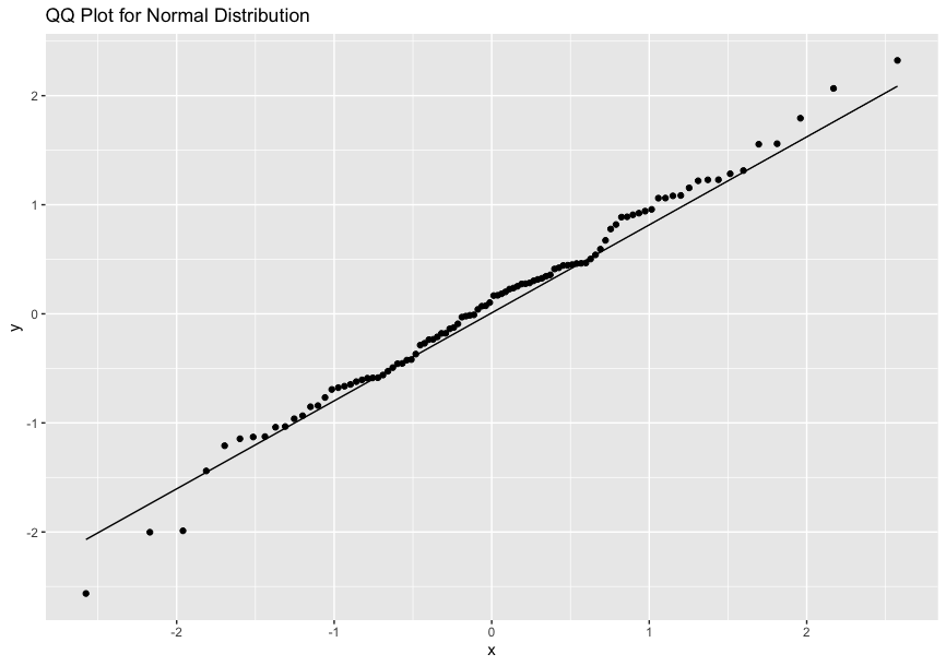
Quantile-Quantile Plot(Q-Q Plot)
The formula for the empirical distribution function is:
\[ F_n(x) = \frac{1}{n} \sum_{i=1}^{n} I(X_i \leq x) \]
According to the law of large numbers, the empirical distribution function approaches the distribution function of the population.
A Q-Q Plot is a scatter plot that compares the empirical distribution to the ideal distribution.
If the points on the Q-Q plot form a linear pattern, the data conforms to the ideal distribution.
Skewness and Kurtosis
\[ skewness = \frac{1}{n} \sum_{i=1}^{n} \left( \frac{x_i - \bar{x}}{s} \right)^3 \]
\[ kurtosis = \frac{1}{n} \sum_{i=1}^{n} \left( \frac{x_i - \bar{x}}{s} \right)^4 - 3 \]
For a normal distribution, both skewness and kurtosis are close to zero.
Goodness of fit test
This test evaluates the goodness of fit between observed and expected frequencies.
Under the null hypothesis , the following value conforms to the distribution:
\[ \chi^2 = \sum \frac{(O_i - E_i)^2}{E_i} \]
Independence test
The null hypothesis for the independence test is:
\[ E_{ij} = \frac{n_{i \cdot} \times n_{\cdot j}}{n} \]
then,
\[ \chi^2 = \sum \frac{(O_{ij} - E_{ij})^2}{E_{ij}} \]
This conforms to the distribution.
Today's study is complete.
統計検定2級の勉強をする話(12)
前回↓
今回は線形モデル分析
今までなんとなーくわかったようなわかってないようなつもりでやっていたので、復習。
こういう時に過去の記事を見るとなんとも言えない気持ちになる。
線形回帰モデル
線形単回帰モデル
\( y = \alpha + \beta_1 x + \epsilon \)
ここで、\( y \)は応答変数(目的変数)、\( x \)は説明変数、\( \alpha \)は切片、\( \beta \)は回帰係数、\( \epsilon \)を誤差項(説明変数のみで説明できない誤差)という。
回帰係数の区間推定
最小二乗法によって求められる回帰係数の推定量\(\hat\beta\)の期待値と分散は
\[ E(\hat{\beta_1}) = \beta_1 \]
\[ \text{Var}(\hat{\beta_1}) = \frac{σ^2}{\sum_{i=1}^{n} (x_i - \bar{x})^2} \]
ここで誤差項の分散\(σ\)は
\[ e_i = y_i - \hat{y}_i \]
\[ \text{SSE} = \sum_{i=1}^{n} e_i^2 \]
\[ \hat{σ}^2 = \frac{\text{SSE}}{n - 2} \]
母集団における誤差項の分散はわからないので、t分布を用いて回帰係数の信頼区間は
\[ \hat{\beta_1} \pm t_{\alpha/2, n-2} \times \sqrt{\hat{σ}^2 / \sum_{i=1}^{n} (x_i - \bar{x})^2} \]
回帰係数のt検定
帰無仮説\(H_0:\beta=\beta_0\)として、自由度n-2のt値を求めて検定を行う。
回帰の現象
ある測定を2回行ったとして、2回目の測定を1回目の測定で回帰分析を行うと、2回目の測定は1回目よりもより平均(回帰係数のぶんだけ)に近づく性質がある。これは1回目と2回目の間に介入した結果とは無関係。これを誤解することを回帰の錯誤という。
線形重回帰モデル
説明変数が2つ以上の時の回帰モデル
重回帰の場合でもSSEを各変数ごとに偏微分して、それぞれ得られた連立方程式を解けば回帰係数を計算可能。
決定係数の欠点
決定係数は応答変数を説明変数がどれだけ説明できるかを表しているが、説明変数の数が増えるほど残差平方和は小さくなり、決定係数は大きくなる。そのため、説明変数の異なるモデル同士の精度を比べることはできない。
そこでその欠点を解消したのが自由度調整済み決定係数
\[ \text{adjusted } R^2 = 1 - \left( \frac{1 - R^2}{n - p - 1} \right) \left( \frac{n - 1}{n} \right) \]
回帰の有意性と回帰係数の検定
回帰モデルに含まれる説明変数の中に応答変数を説明できる変数があるかどうか、すなわち、
\[ H_0: \beta_1 = \beta_2 = \ldots = \beta_p = 0 \]
という帰無仮説のもとで、平方和を自由度で割った値はχ二乗分布に従うので、
\[ \frac{ \frac{1}{p} \sum_{i=1}^{n} (\hat{y}_i - \bar{y})^2 }{ \frac{1}{n-p-1} \sum_{i=1}^{n} (y_i - \hat{y}_i)^2 } \]
はF分布に従う。
2つのモデルのどちらかが優れているかを検定するにはモデルが階層的になっている必要があり、その際の帰無仮説は
\[ H_0: \beta_j = 0 \]
で、t統計量は
\[ t = \frac{\hat{\beta}_j}{SE(\hat{\beta}_j)} \]
信頼区間は
\[ \hat{\beta}_j \pm t_{\alpha/2} \times SE(\hat{\beta}_j) \]
(自由度はn-k-1)
*多重共線性
説明関数間の相関が強い場合、回帰係数の推定制度が悪くなり、解釈が困難になること。
相関係数の区間推定と検定
母集団の相関係数の推定
標本の相関係数rの確率分布はnが極めて大きい場合以外は母集団の相関係数に影響を受けて非対称になる。
そこで、Fisherのz変換と言われる
\[ z = \frac{1}{2} \ln \left( \frac{1 + r}{1 - r} \right) \]
が対称になることを利用する。
このzは
\[ E(z) = \frac{1}{2} \ln \left( \frac{1 + \rho}{1 - \rho} \right) \]
\[ \text{Var}(z) = \frac{1}{n-3} \]
に従う。このことから
zの95%信頼区間は
\[ z \pm z_{\alpha/2} \times \sqrt{\frac{1}{n-3}} \]
母集団の相関係数 \( \rho \) の95%信頼区間は双曲線正接関数である
\[ {\rho} = \frac{e^{\rho} - e^{-\rho}}{e^{\rho} + e^{-\rho}} \]
から計算できる。
無相関性の検定
帰無仮説 \(H_0:{\rho}=0\)を考える。
これは、共分散が0 であることと同義であり、単回帰モデルを考えると、
回帰係数の区間推定を相関係数に対する検定としても利用可能である。
分散分析モデル
一元配置分散分析
3つ以上の母集団に対して検定を行う場合、第1種過誤の可能性が増えるためt検定は適切でない。
1つの質的変数(因子)のカテゴリを水準と呼び、各水準内の誤差変動と水準間の平均の変動を比較することを分散分析という。
\[ Y_{ij} = \mu + \alpha_i + \epsilon_{ij} \]
ここで、μは一般平均、αはi群の効果という。
水準の母平均が等しいという帰無仮説において、
\[ F = \frac{\frac{\text{SSB}}{k - 1}}{\frac{\text{SSW}}{N - k}} \]
はF分布に従う。SSBは水準間平方和、SSWは群内平方和。
これによって3つ以上の母集団の平均の検定を行うことができる。
2元配置分散分析
因子が2つになる場合、それぞれの水準の組み合わせによって異なる観測値を取るので、モデルとしては、
\[ Y_{ijk} = \mu + \alpha_i + \beta_j + (\alpha \beta)_{ij} + \epsilon_{ijk} \]
となる。
二次元配置データに対しての平方和の分解は
となり、AとBそれぞれの主効果と2つの因子の交互作用、そして残渣平方和になる。
それぞれの項に対して検定を行えば、特定の因子の主効果及び交互作用の検定ができる。
今日はここまで、分散分析が正直まるでわかってない。
Study for Statistics Test Level 2 (11)
previous page↓
Today's study is on "Hypothesis testing".
Hypothesis Testing
Null Hypothesis and Alternative Hypothesis
The null hypothesis asserts that there is no significant difference or effect.
When a rare probability event is observed under the null hypothesis, the hypothesis is considered false.
If the probability of the event is smaller than the significance level (commonly set at 0.05 or 0.01), the null hypothesis is rejected.
The hypothesis that opposes the null hypothesis is termed the alternative hypothesis.
If the null hypothesis is rejected, it suggests the alternative hypothesis is correct. However, if the null hypothesis is accepted, it doesn't prove its correctness.
Alternative hypotheses can be two-sided or one-sided.
Test Statistic and Rejection Region
The mean or ratio of a sample used in testing is termed the "test statistic."
If there's a range within which the null hypothesis is rejected for the test statistic, this range is called the rejection region (opposite of the acceptance region).
The p-value represents the probability that the test statistic will have a value rarer than the observed value.
Classification of Hypotheses
Hypothesis testing methods can be classified as follows:
 One Sample Problem
Population variance known (z-test)
- Two-sided alternative hypothesis
\[ \bar{X} < \mu - 1.96 \times \frac{σ}{\sqrt{n}} \] \[ \bar{X} > \mu + 1.96 \times \frac{σ}{\sqrt{n}} \]
- one-sided alternative hypothesis
\[ \bar{X} > \mu + 1.645 \times \frac{σ}{\sqrt{n}} \]
*level of significance=0.05
Population variance unknown (t-test)
Use unbiased variance in place of variance when population variance is unknown.
This formula doesn't follow a normal distribution but a t-distribution.
Two Sample Problem
Population variance known (z-test)
- Paired
The z-test is conducted similarly to the one-sample problem. - Unpaired
\[ \begin{align*} Z &= \frac{(\bar{X}_1 - \bar{X}_2)}{\sqrt{\frac{σ_1^2}{n_1} + \frac{σ_2^2}{n_2}}} \\ \end{align*} \]
Population variance unknown(z test)
- When population variances are equal
\[ \begin{align*} t &= \frac{(\bar{X}_1 - \bar{X}_2)}{s_p \sqrt{\frac{1}{n_1} + \frac{1}{n_2}}} \\ s_p &= \sqrt{\frac{(n_1 - 1) s_1^2 + (n_2 - 1) s_2^2}{n_1 + n_2 - 2}} \\ \end{align*} \]
- When population variances are unequal(Welch's test)
\[ \begin{align*} t &= \frac{\bar{X}_1 - \bar{X}_2}{\sqrt{\frac{s_1^2}{n_1} + \frac{s_2^2}{n_2}}} \\ \nu &\approx \frac{\left(\frac{s_1^2}{n_1} + \frac{s_2^2}{n_2}\right)^2}{\frac{(s_1^2/n_1)^2}{n_1-1} + \frac{(s_2^2/n_2)^2}{n_2-1}} \\ \end{align*} \]
Today's study session has concluded.
統計検定2級の勉強をする話⑩
前回
最近ただの統計勉強ブログと化していてプログラミング全然やってない。
今日は1標本問題と2標本問題について
1標本問題
母集団が1つで1つの標本を抽出したときにその母数について推測すること。
正規分布の母平均の推定
母分散が既知の時
前回やったように、95%信頼区間を用いて母平均が推定される。
\[ \mu \pm z \left( \frac{σ}{\sqrt{n}} \right) \]
母分散が未知の時
サンプル数が少ない場合はt分布を用いて、
\[ \bar{x} \pm t_{\alpha/2, n-1} \left( \frac{s}{\sqrt{n}} \right) \]
とする。
自由度が高ければt分布は標準分布に収束するので、
サンプル数が多ければ、母分散の代わりに不偏分散の平方根を用いることができる。
母分散の区間推定
正規分布からの標本に対して、 標本平均との偏差の2乗の和を分散で割ったものは
分布に従う。
\[ \left( \frac{(n - 1) σ^2}{\chi^2_{(1 - \alpha/2, n-1)}} , \frac{(n - 1) σ^2}{\chi^2_{(\alpha/2, n-1)}} \right) \]
*標準偏差に関しては平行根を取ればおk
母比率の推定
母数N数が多い場合には、Nのうちxが生じる数は二項分布に従うと考えられる。
\[ \hat p = \frac{x}{n} \]は不偏推定量で、期待値と分散は
\[ E(\hat p) = p \]
\[ \text{Var}(\hat p) = \frac{p(1-p)}{n} \]
中心極限定理より、二項分布はNが多ければ標準正規分布に近づき、大数の法則でpを\(\hat p\)に近似して、95%信頼区間は
\[ p \pm z \sqrt{\frac{p(1-p)}{n}} \]
で表せる。
*ただし、二項分布と考えられるのは復元単純無作為抽出(重複を排除しない方法)のみで、実際の抽出に多い非復元単純無作為抽出では超幾何分布に従う。
2標本問題
母集団が2つの時の区間推定
母平均の差の区間推定
母平均の差の推定量として標本平均の差を用いることができる。
それぞれの標本平均が正規分布に従うことから、標本平均の差も正規分布\(( \mu_1 - \mu_2 \),\(\frac{σ_1^2}{n_1} + \frac{σ_2^2}{n_2}) \)に従う。
よって母分散が既知の場合は標準正規分布を用いて区間推定ができる。
母分散が未知だが等しい時は、それぞれの不偏分散から合成されたプールした分散
\[ s_p^2 = \frac{(n_1 - 1) s_1^2 + (n_2 - 1) s_2^2}{n_1 + n_2 - 2} \]
に置き換えた確率変数がt分布に従うとして区間推定できる。
対応のある2標本の区間推定
2組の標本に対応関係がある時は上述の方法は使えない。
平均の差に関する区間推定は、その差を1標本として平均と分散を用いれば良い。
母分散の比の区間推定
それぞれの母集団を標本集団に対して、
\[ \frac{\sum_{i=1}^{n} (x_i - \bar{x})^2}{σ^2} \]
はχ2乗分布に従う。
独立した確率変数がχ2乗分布に従うとき、
\[ F=\frac{W1/N1}{W2/N2} \]
はF分布に従うので100(1-α/2)%点から95%信頼区間を求められる。
本日はここまで。むずい。問題が解けなくなってきた。。。
Study for Statistics Test Level 2 (9)
previous page↓
Today's study is on "Inferential Statistics".
Population and Sample
A population refers to the entire set under analysis.
A sample is a subset taken from the population.
A sample survey aims to infer population characteristics from the sample.
Design of Study
Experimental Study
An experimental study allows researchers to determine the conditions.
Three principles, often attributed to Fisher, are crucial in experimental studies:
Fisher's Three Principles:
- Randomization
- Replication
- Local control
Observational Study
An observational study is one where researchers cannot set the conditions.
In observational studies, randomization is excluded from the three principles, leading to potential selection bias.
Methods of Sampling
Simple Random Sampling
Every individual has an equal probability of being selected, and every combination is equally likely.
Systematic Sampling
In systematic sampling, individuals in the population are numbered, and selections are made at regular intervals.
Stratified Random Sampling
Stratified random sampling involves selecting samples from specific subgroups, such as gender, age, or occupation. The goal is to increase accuracy by reducing variability.
Multistage Sampling
Multistage sampling involves selecting samples at various stages based on different criteria. While this method simplifies the sampling process, it may compromise accuracy.
Point Estimation and Interval Estimation
Point Estimation
Point estimation refers to using a single value from the sample as an estimate.
Order Statistic
When samples are arranged in order, it's termed "order statistic."
If the distribution is symmetrical, the median equals the mean.
Trimmed Mean
A trimmed mean is calculated by excluding an equal number of the highest and lowest values from the sample.
Consistency and Unbiasedness
An estimator should be consistent and unbiased.
Consistency means that as the sample size grows, the estimator approaches the parameter value.
Unbiasedness implies that the expected value of the estimator matches the parameter, regardless of sample size.
For instance, sample means or unbiased variances are unbiased estimators.
Standard Error
When comparing estimators, the one with less variability is superior.
This variability is termed "standard error," which uses the variance of the sample.
Interval Estimation
Interval estimation provides a range within which the estimator lies, based on two values from the sample.
For a normal distribution, the following formula indicates that the population mean lies within this range with 95% probability:
Today's study has concluded.